2.1 Does brand has an impact on smartphone prices?
Authors: Agata Kaczmarek, Agata Makarewicz, Jacek Wiśniewski (Warsaw University of Technology)
2.1.1 Abstract
Mobile phone became indispensable item in our daily life. From a simple device enabling contacting other people, it developed into a tool facilitating web browsing, gaming, creating/playing multimedia and much more. Therefore, the choice of phone is an important decision, but given the wide variety of models available nowadays, it is sometimes hard to choose the best one and also easy to overpay. In this paper, we analyze the phone market to investigate whether the prices of the phones depend only on their technical parameters, or some of them have an artificially higher price regarding the possessed functionalities. Research is conducted on the phones dataset, provided by the lecturer, containing prices and features of different phones. As a regressor, Random Forest from package ranger (Wright and Ziegler 2017a) was chosen. Given the type of the model (black box i.e. non-interpretable), we use Explainable Artificial Intelligence (XAI) methods from DALEX (Przemyslaw Biecek et al. 2021) and DALEXtra (Maksymiuk and Biecek 2020a) packages, for both local and global explanations, to interpret its predictions and get to know which features influence them the most, and raise (or lower) the price of the phone.
2.1.3 Methodology
Data description
The research was carried out on the phones dataset provided by the lecturer i. e. data frame with prices and technical parameters of 414 phones. It contains ten explanatory variables and one target variable (price), therefore we deal with regression task. The sample of the data is presented below (2.1).
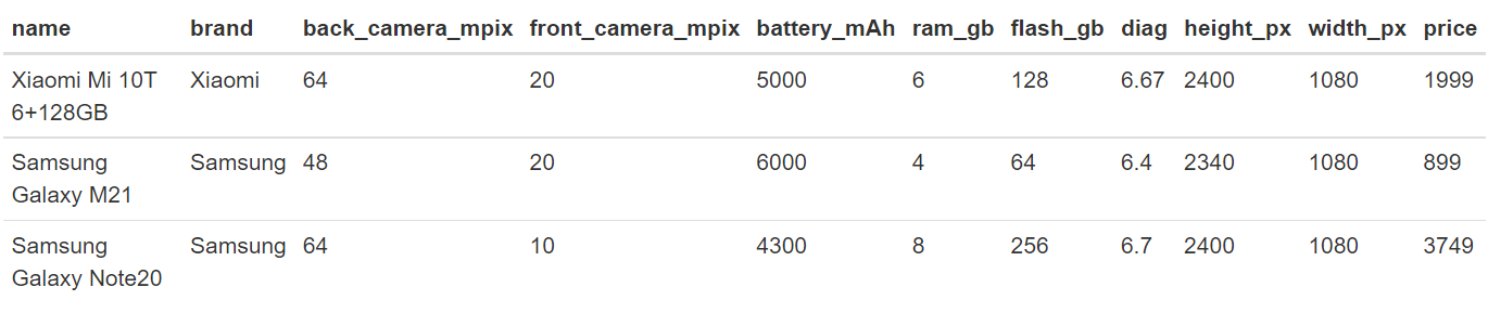
Figure 2.1: Sample of the data
Exploratory Data Analysis and data preprocessing
At the beginning of our research, we conducted Exploratory Data Analysis to get a better understanding of the data we deal with. We mainly focused on the target variable and its distribution versus explanatory ones to identify potential influential features for our prediction. Below we present some results important for further work.
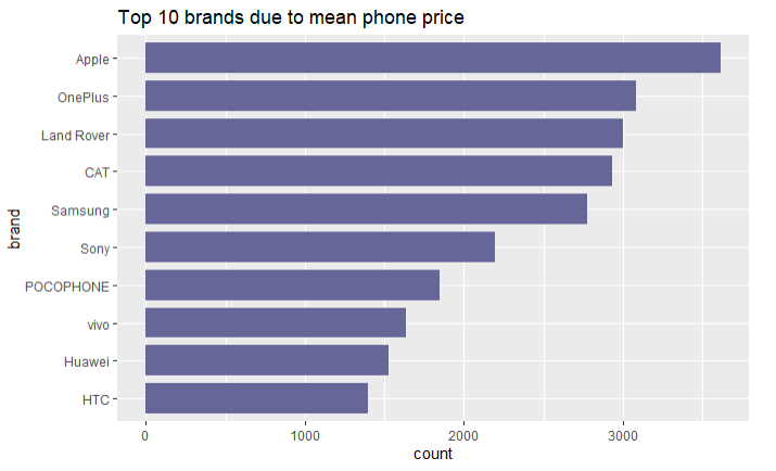
Figure 2.2: Ten brands with the highest mean price of the phone among the observations from the dataset.
Analyzing brands by the mean price of the phones produced, there can be identified a distinct leader, which is an Apple company. On average, a phone from it costs more than 3500 PLN. In the top 10 brands, we can also see common ones such as Samsung or Huawei.
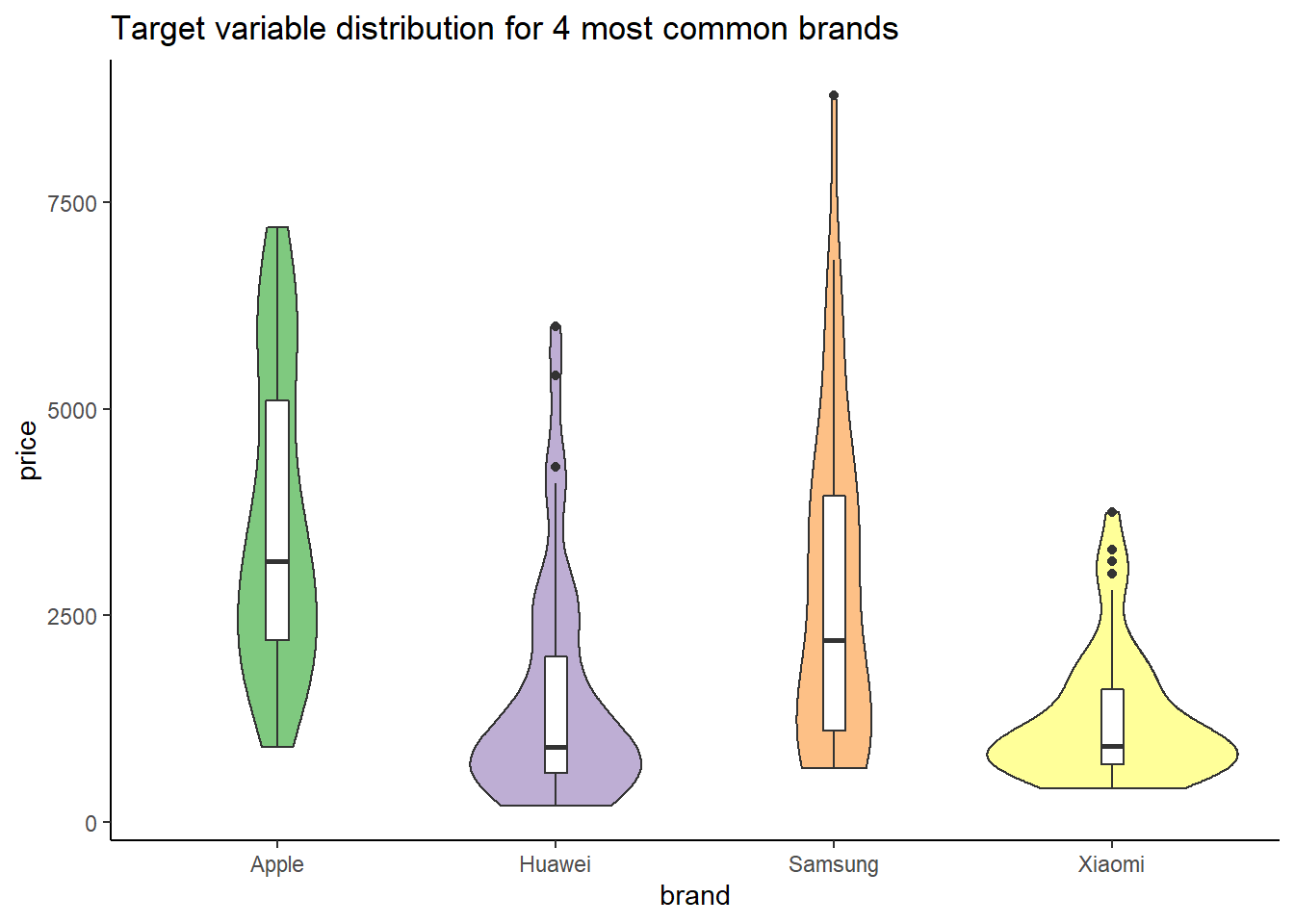
Figure 2.3: Phone price distribution for 4 most common brands among the observations from the dataset.
On the plot above (2.3) we can identify some outliers in terms of price, especially a phone made by Samsung company, which costs 9000 PLN. Concerning the Xiaomi brand, we can observe that despite being a popular choice, the price of a single phone is relatively low - no phones are exceeding 4000 PLN. As for the Apple products, conclusions from the plot above are confirmed.
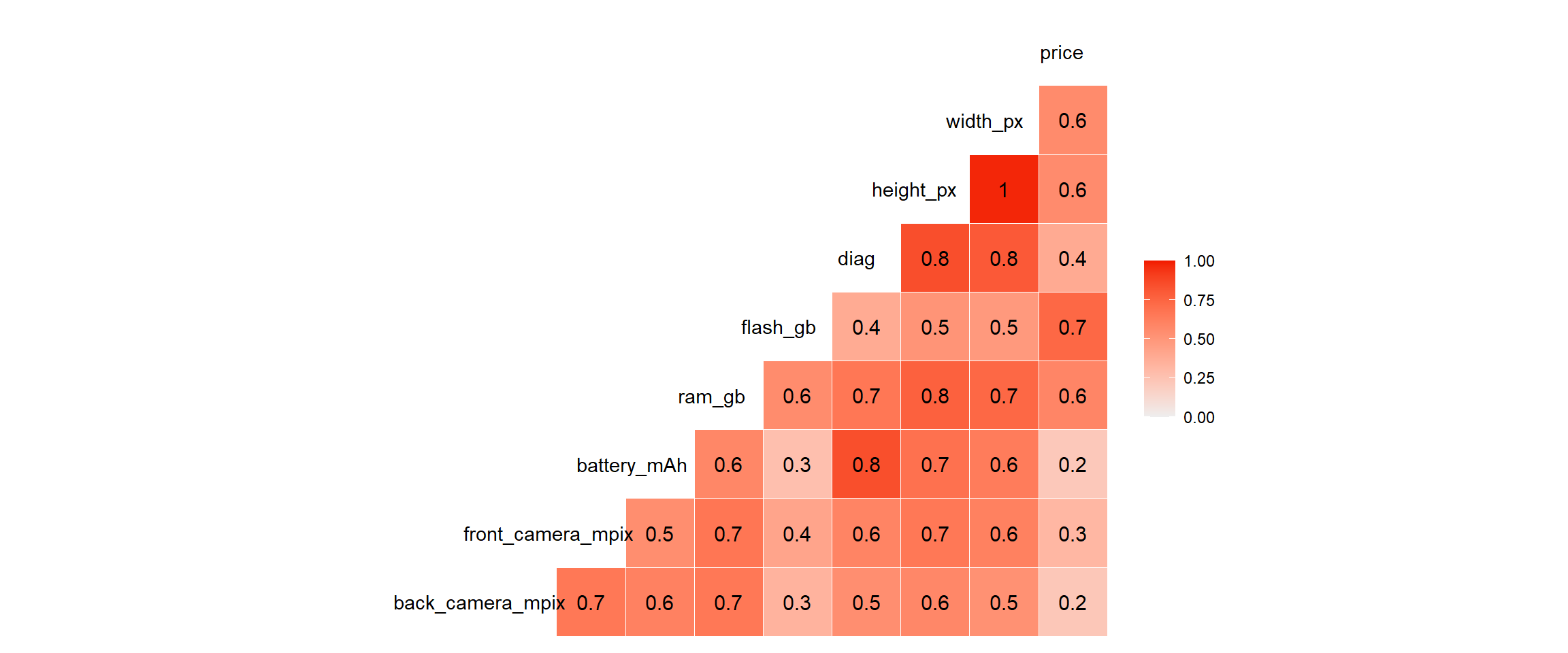
Figure 2.4: Correlation matrix for numeric features
Based on the partially presented EDA, we needed to conduct simple data preprocessing before modelling. The following steps were executed:
- handling missing values: Two features containing missing values were identified; both related to camera parameters (
back_camera_mpix,front_camera_mpix). Those values turned out to be meaningful, as they mean that the given mobile phone has no camera (back or front). Given that information, NAs were imputed with a constant value - 0. - removing outliers: Based on features distribution, some extreme values were identified in the dataset’s explanatory variables (
back_camera_mpix,front_camera_mpix,battery_mAh,flash_gb,price), which would weaken the model’s performance. Therefore they were removed. - dealing with unimportant and correlated features: The variable
namehas been omitted, because it was practically unique in the dataset and naturally connected to thebrandfeature. Moreover,height_pxandwidth_pxwere deleted due to their strong correlation with thediagfeature (and with each other) (2.4); this feature was considered as a sufficient determinant of the phone’s dimensions.
Models
The next step after EDA was creating prediction models. To compare results and find the best model for mentioned data, there were created 3 models: Random Forest from ranger package (Wright and Ziegler 2017a), XGBoost from mlr package (Bischl et al. 2016a) and SVM, also from the mlr package. For each of them, training using 5-fold cross-validation was performed. SVM and XGBoost models cannot be trained using categorical variables so variable brand needed to be target encoded in these cases. There were used two measures to compare models results: Root Mean Squared Error (RMSE) and Mean Absolute Error (MAE). The results are presented in the table below.
| rmse | mae | |
|---|---|---|
| ranger | 547 | 295 |
| xgboost | 1515 | 1033 |
| svm | 678 | 376 |
The presented results point, that the ranger model is the best choice. This model was used in further analysis.
2.1.4 Results
Ranger model results have been analyzed using Explainable Artificial Intelligence methods. Following paragraphs present local and global explanations.
Local explainations
In the first step of our XAI, the focus was on instance level explanations - analysis of single predictions and how each feature influences their values. Every local explanation method (Staniak et al. 2018) takes one observation and draws the results for it. The results for each observation can differ greatly from the results for the other observation. Thanks to it we can eg. compare two observations and the influence of various features on the prediction. However, this causes that we cannot assume general ideas for a whole data set based on results from local explanations. Therefore below we present only the most interesting observations found during the research. Breakdown (Staniak and Biecek 2018a), SHAP (Scott M. Lundberg and Lee 2017), Lime (Ribeiro et al. 2016b) and Ceteris Paribus (Przemyslaw Biecek and Burzykowski 2021a) profiles were used to show dependencies and draw conclusions. Observations below were grouped into pairs to show how identical parameters, but different brands can lead to totally different prices or vice versa.
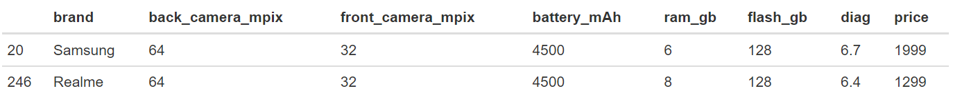
Figure 2.5: Two phones (Samsung and Realme) from data set, which have similar features, various prices.
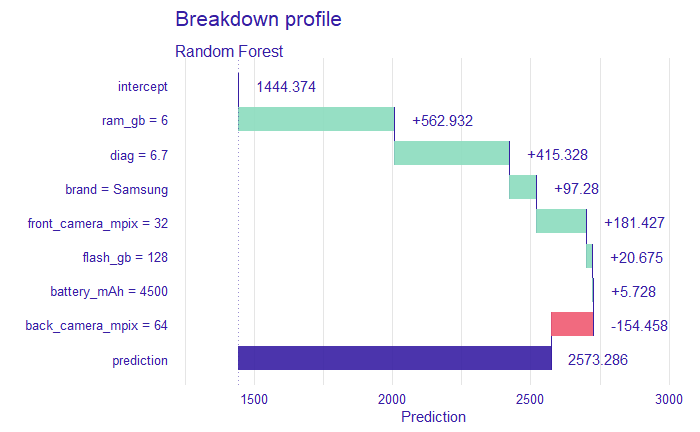
Figure 2.6: Breakdown profile plot drawn for observation 20 - Samsung phone from above table.
Figure 2.7: Breakdown profile plot drawn for observation 246 - Realme phone from above table.
The above-shown Breakdown (Staniak and Biecek 2018a) profiles help answer a common question: which variable contributes to the prediction the most. It is of course only one of the possible solutions, some of the others are presented further. This method shows the decomposition of the prediction done by model, most important features plotting the highest. Next to each feature, there is a number showing the value of the influence of the feature on the prediction. We can separate features with positive (green bars) and negative (red) influence.
Shown above two observations (2.5) vary three features - ram_gb, brand and diag. It is visible on these two Breakdown charts (2.6, 2.7) that Samsung has a bigger diagonal, but less RAM GB and according to the model is more expensive by 200. However, this difference, in reality, is higher, Samsung is more expensive by 700. There are also differences in the impact of features - in first batter_mAh has a positive impact and in the second negative. In the first case for model the most important were ram_gb, diag and brand (in this order), in second ram_gb, brand and front_camera_px. The question is, whether in reality brand does not have a bigger impact on price than shown here?
Figure 2.8: Two phones (Apple and Motorola) from data set, Motorola has better features and is cheaper.
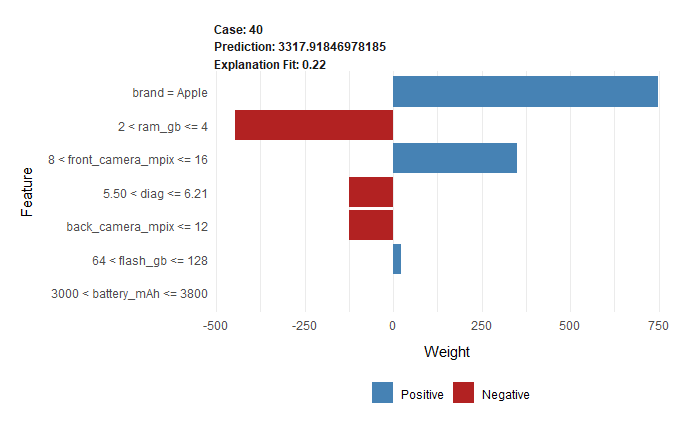
Figure 2.9: Lime plot drawn for observation 40 - Apple phone from above table.
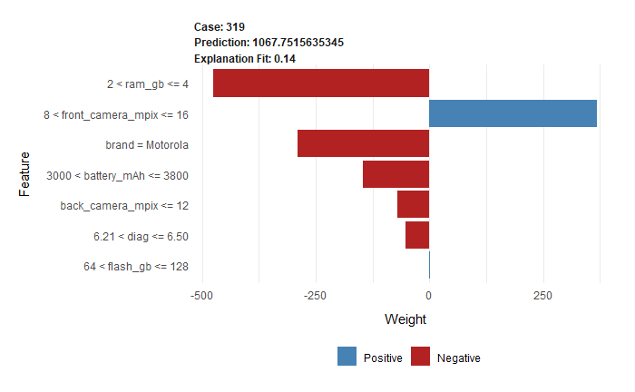
Figure 2.10: Lime plot drawn for observation 319 - Motorola phone from above table.
The above-shown Breakdown profile is most suitable for models with a small number of features. However, it sometimes happens that we need to use more features and Breakdown is not the best choice. Better is Lime (Local Interpretable Model-agnostic Explanations) profile (Ribeiro et al. 2016b). It is one of the most popular sparse explainers, which uses a small number of variables. The main idea of it is to change the complicated black-box model into approximated glass-box one. In this situation, the second one is much easier to interpret. On the Lime plots, we can also see the influence of the features on the final prediction, with division (shown as various colours) on positive and negative.
On LIME plots (2.9, 2.10) two phones, which have similar values in many features (2.8), in two (battery_mAh and diag) second phone (2.10) has better values than first one (2.9). Even though the price of the first phone is three times higher according to our model. The only difference not mentioned above between them is a brand - the first one is the iPhone. That seems to be a conclusion consistent with reality.
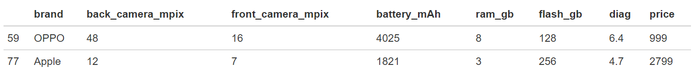
Figure 2.11: Two phones (OPPO and Apple) from data set, Apple is about three times more expensive having similar features.
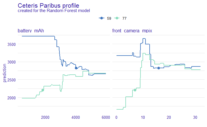
Figure 2.12: Ceteris paribus profile plot drawn for observations 59 and 77 (shown in above table).
Above mentioned profiles showed the various influence of features on the prediction and the comparison between them. Ceteris Paribus profile (Przemyslaw Biecek and Burzykowski 2021a) shows the effect on the model’s predictions made by changes in the value of one individual feature, while the rest of them held constant. These profiles help us understand how changes in one feature affect the prediction of the model for all of the features.
Ceteris Paribus profile (2.12) shows different influence of some features concerning two mobile phones (2.11). The biggest contrast we can observe in the case of battery_mAh, which lowers the price significantly in the case of OPPO phone, and increases when it comes to Apple one, leading to the same prediction for both if the value exceeds 5000 mAh. It is quite surprising because in the case of the first one such battery parameters should lead to a bigger price. Another difference which can be observed in front_camera_mpix influence - whereas above ~ 15 Mpix we reach similar price, for smaller values it causes prediction’s increase for Apple, and steady value for OPPO (for both peaks around 10 Mpix value). Once more those impacts are unexpected because the OPPO phone has a much better front camera.
Global explanations
In the second step of our XAI analysis, we focused on dataset level explanations - those concerning not a single observation, but all of them. Global methods let us gain a better understanding of how our model behaves in general and what influences it the most. We perform an analysis of all predictions for the dataset together to find out how each feature affects their average value. The methods used for this purpose are Permutation-based Variable Importance (Feature Importance) (A. Fisher et al. 2019b) and Partial Dependence Profile (PDP) (Friedman 2000b).
Feature Importance is a method assessing which variables have the most significant impact on the overall model prediction. The idea of it is to evaluate a change in the model’s performance in a situation when the effect of a given variable is omitted. This simulation is achieved by resampling or permuting the values of the variable. If a given feature is important to our model, then we expect that after those permutations the model’s performance will worsen; therefore the greater the change in the model’s performance, the bigger is the importance of a feature. The calculations, which results are presented below, were performed for 5000 permutations, to achieve stability.
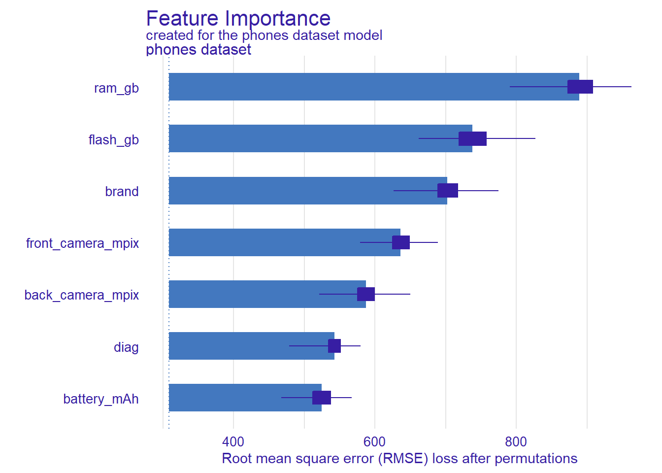
Figure 2.13: Feature importance explanation for the phones dataset variables. Blue thick bars correspond to RMSE loss after permutations. Dark blue bars represent boxplots for 100 bootstrapped explanations.
According to the plot (2.13), the most important variables for the model are ram_gb, flash_gb and brand, with visible domination of ram_gb. After these, the next variables in terms of impact are the camera-related ones, then diag and battery_mAh. These observations coincide with the conclusions drawn from local explanations (2.6, 2.7) - for single predictions, brand and memory-related variables were also very important and had a significant impact on the price of the phone, and camera-related were next. Whereas those previous results could be a coincidence, and true only for those 2 chosen observations, now we are ensured that those conclusions are adequate for the whole dataset. Moreover, these results confirm also our intuition. Memory parameters are arguably the most important phone’s technical parameters and the high position of brand on the chart shows, that, probably in the case of the bigger companies, the prices of the phones are likely to be biased with regard to their parameters.
In order to perform further analysis of the model’s behaviour on the global level, Partial Dependence Profile was used. The general idea underlying the construction of PDP is to show how the expected value of model prediction behaves as a function of a selected explanatory variable. Comparison of these profiles may give additional insight into the stability of the model’s prediction.
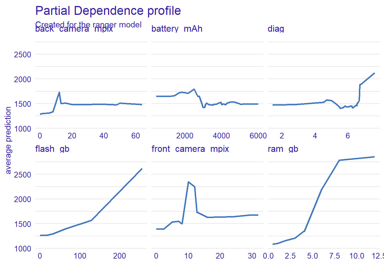
Figure 2.14: Partial Dependence Profile (PDP) explanation for numeric variables in phones dataset. Blue lines represent variable (horizontal axis) and price (vertical axis) dependence.
The plot above (2.14) confirms observation from the previous plot (2.13), presenting a strong dependency between our target (price) and memory parameters. For the variables flash_gb and ram_gb, we can observe similar profiles - as the value of the variable increases, the estimated price of the phone increases. In the case of the front_camera_mpix variable, there can be seen an unnatural behaviour near 10-12 mpx, suggesting that phones with these specific parameters are the most expensive. We have already observed this characteristic behaviour in previous analyzes for single predictions (2.12). In order to investigate this anomaly, the further analysis presented below was performed.
| Number of phones | |
|---|---|
| Apple | 21 |
| Motorola | 3 |
| Samsung | 14 |
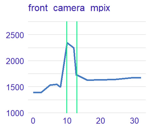
Figure 2.15: Results of the research explaining front camera mpix PD profile anomaly. The table above presents the number of phones grouped by brand having from 10 to 12 front camera mpix value. The PDP plot below the table presents the front camera mpix PD profile with marked 10 and 12 values.
The research proved that phones having from 10 to 12 megapixels in their front camera are mostly represented by expensive brands like Samsung and Apple in the phones dataset. This leads to the conclusion, that in this case, it was the brand that influenced the phone’s price, not the quality of the front camera.
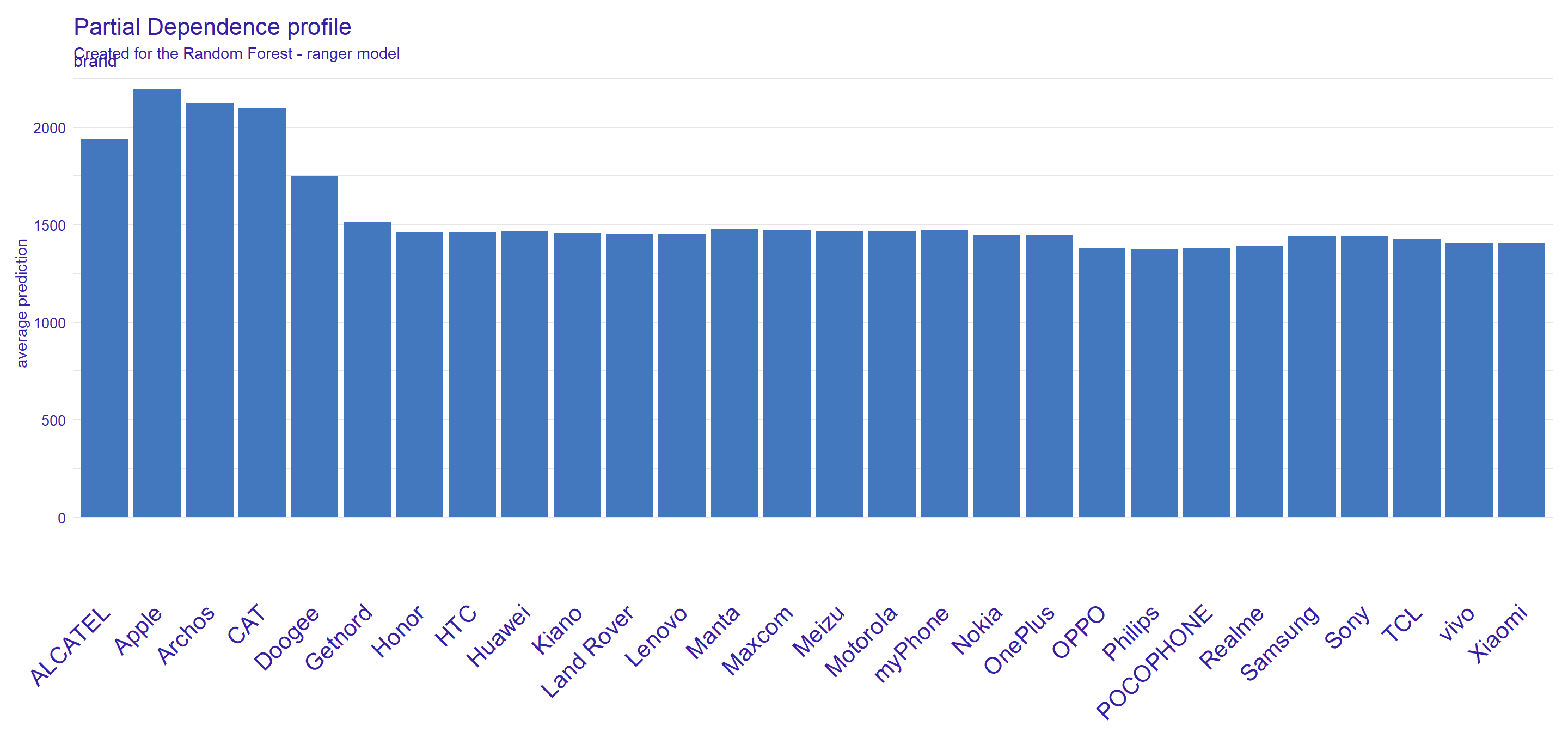
Figure 2.16: Partial Dependence Profile (PDP) explanation for brand variable in phones dataset. Blue bars represent the average predictions for each brand in the dataset.
Partial Dependence Profile (2.16) looks slightly different for the brand variable because it is a categorical variable. Surprisingly, this plot presents a weak brand name impact on price, unlike previous plots: (2.14) and (2.13) - for most brands we observe a very similar prediction value. Brands that increase the price are Apple, Archos, and CAT, but only one of those brands (Apple) is a big phone company, however, for this brand, we actually already observed “unexpected” high prices of phones disproportionate to their parameters (. CAT brand is represented by three phones wheres Archos appears in the dataset only once. That leads to the conclusion, that their PD profile might not be stable.
2.1.5 Summary and conclusion
The data set explored in the above research included only a small number of features, even though the obtained results seem to be realistic from the customer’s point of view. The evaluation of our model revealed expected results.
To summarize, according to all explanations shown above, there are several conclusions, which can be drawn. The biggest impact on the predicted price for the model had features describing brand, RAM storage and internal memory size. We believe that the most expensive brands such as Samsung and Apple have biased prices because they are higher than predicted by the model. What is important to highlight is that these conclusions were made for this specific data set, which had only eleven features at the beginning.
The constantly changing market of mobile devices is unexplored and further research based on more complicated models and bigger data sets, with more features, could be beneficial to both customers and companies. These data sets could contain information about processor and durability, which seem to be important features for customers, yet were not included in our data set. Also, phone prices vary across continents and countries, so the results will be different.