6.4 Rashomon sets on death prediction XGB models using MIMIC-III database
Authors: Ada Gąssowska, Elżbieta Jowik (Warsaw University of Technology)
6.4.1 Abstract
In many health-related realms, causality, i.e. a thorough understanding of which input parameters are relevant to an outcome and understanding how particular features affect the prediction overall is especially noteworthy. Since the variable importance is only an oversimplified estimation represented through a single value, taking it as the only criterion may be a misconception.
The task that we reproduced was an in-hospital mortality prediction.
A specific critical care database, which is MIMIC III, had was used to create a group of classifiers to be confronted and the AUC was a baseline measure against which it was built.
The aim of this article is to provide an empirical comparison of ensemble predictive models (i.e. XGBoost), which all perform roughly equally well (i.e. so called Rashomon set), with respect to: (1) predictions validity, (2) the order and grounds of the splits performed (feature importance, partial dependence) , (3) parameter grids similarity degree. For the research purposes we used PCA method, so that we explained the factors that influenced their final behavior.
On the basis of the conducted research, we conclude that the degree of model similitude strongly depends on the choice of the comparative criterion and the resemblance relation is not transitive, that is, the similarity of models with respect to one criterion does not imply alikeness with regard to another. Furthermore, in general, XGB models from the Rashomon set may be grouped into clusters in the reduced parameter space.
6.4.3 Methodology
6.4.3.1 Experiment settings
The study focused on models generated by XGBoost algorithm which is an implementation of gradient boosted decision trees designed for speed and performance. The algorithm performs well both on regression and classification tasks.
Since mortality prediction is a classification problem, cognately to the authors of the reproduced article intentions, we used the XGBClassifier() function from the XGBoost Python package. To create and examine a set of Rashomon models for a given dataset and task, we created a value grid for nine hyperparameters: max_depth, learning_rate, subsample, colsample_bytree,colsample_bylevel, min_child_weight, gamma, reg_lambda and n_estimators. The distributions of the hyperparameters we tuned were taken from the (Probst et al. 2019) paper.
With the random search use, we obtained 100 models, for which the learning process on a data set and a 5-fold cross-validation were carried out. We analyzed the variability of the number of models in the Rashomon Set (set of best models) depending on the values of theta parameter which is the maximum difference between the best model’s AUC score, and the AUC score of the models accepted into Rashomon Set.
6.4.3.2 Analysis workflow
Taking into account the degree of similarity of the results of individual models in terms of the adopted metrics, we decided to select the best 20 for analysis in the remainder of this study. Then, for the three features that occurred in in every model’s top five, we analyzed PDP plots, which showed how that particular variable’s value change affected the prediction of each model.
In the next step, we studied the resemblance of the predictions of the models from the Rashomon Set, by using the accuracy score between each pair of models which described how many of the class predictions were the same for the two of them. We also computed the actual accuracy score between each model’s prediction and the real response variable. As our data was imbalanced, we checked the F1 score of each model, and as the results quite differed we used PCA (Principal Component Analysis) to see if the models with high F1 score differ in terms of hyperparameters from the models for which the score was low.
6.4.4 Results
It should be mentioned that almost all of the 100 checked models achieved quite similar AUC scores, and for the theta 0.03, almost half of the models were included in the Rashomon Set. Rashomon sets size variability due to theta parameter value change are shown in the table below:
| Theta | Number of models in Rashomon set |
|---|---|
| 0.005 | 3 |
| 0.01 | 12 |
| 0.015 | 24 |
| 0.02 | 30 |
| 0.025 | 36 |
| 0.03 | 44 |
For the rest of experiments we decided to choose 20 best models, where difference of AUC scores between the first and the twentieth was equal to 0.012 and the best score achieved was 0.906.
6.4.4.1 Predictions resemblance and grounds of the splits performed similarity context .
For each model we analysed the features importances and chose 5 most critical variables, which were assigned a score from 5 (most important variable) to 1 (the fifth most important variable). All remaining features were given a score of 0. The scores achieved by features which were included in at least one model’s top five most important variables are presented on Figure 1:
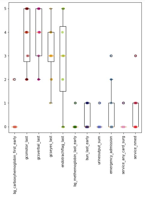
Figure 1.: The most important features scores distributions.
Quite interestingly those three features all happen to be related to Glasgow Scale which is a clinical scale used to reliably measure a person’s level of consciousness. The variable gcseyes_last describes the dynamic of the patient’s eyes opening, gcsmotor_last - the dynamic of the patient’s motoric movement and gcsverbal_last - the person’s verbal dynamic. For all these characteristics, the higher the value, the better the patient’s condition.
Figures Figure 2 to Figure 4 present the PDP charts for these three variables for each of the twenty models alongside their histograms. On each chart, almost all of the lines presented seem to be pararel, which means that the models treat the variables in a similar way.


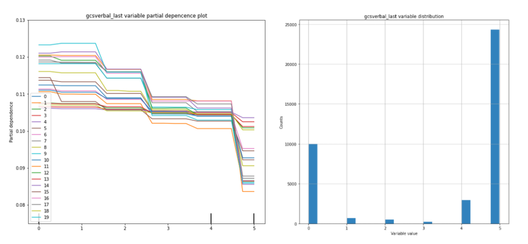
Figure 4: Partial dependende and histogram charts for gcsverbal_last variable .
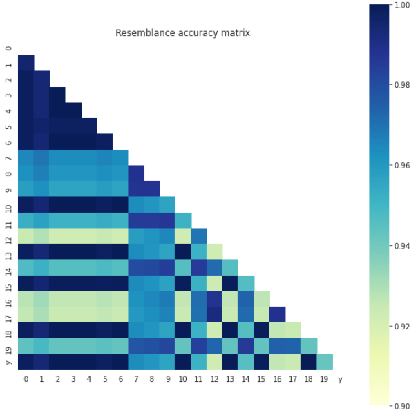
Figure 5: Models pairs resemblance and validity calculated with respect to the Accuracy measure.
As most of the model-resemblance measures we used in the study were based on the comparison of the models’ independent variables and predictions validities, in the final stage of the research we decided to confront the conclusions drawn so far using a different approach, which was models’ parameter grids similarity extent examination. We aimed to conclude on how much is the Rashomon set’s content and volume impacted by the measure according to which it was created.
6.4.4.2 The study on models parameter grids similarity.
The study on models parameter grids resemblance degree was conducted in groups built with respect to the F1 measure. The results came out quite interesting as eleven out of all twenty models obtained scores of over 0.95 and the other 9 had scores lower than 0.8, some of which achieved score as low as 0.5. This created the question if these two groups of models differed in the context of hyperparameters values. To analyse that, we used Pricipal Component Analysis to plot the models on the 2D plot. The results may be seen on Figure 6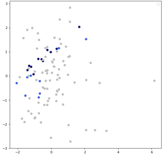
Figure 6: Obtained PCA results - each point color corresponds to the Rashomon set the model belongs to and F1 score value it obtained.
The models represented by grey points are the 80 models that did not belong to the Rashomon Set, while these represented by blue points did - for models marked with a dark the F1 score value was over 0.9, for the ones exemplified with light blue points, F1 score was under this value. Although it is hard to define clear clusters, it seems that there is a split. Also models with higher F1 score values seem to be arranged in a shape similar to a line, thus it may mean that their hyperparameters have some things in common.
6.4.5 Conclusions
The purpose of this exploration was to provide and formalize a comprehensive, empirical comparisons of a Rashomon set of ensemble predictive models that may differ in terms of predictions validity, the variables impact and parameter values similarity.The conducted study revealed both certain similarities and clear discrepancies between the individual criteria explored.
Since the importance of a feature is the increase in the prediction error of the model after permuting/shuffling the given feature values and PDP plots show the marginal effect of one predictor on the response variable, by definition, these criteria are closely related. Therefore the similarity of the impacts of the significant variables on the prediction, indicated by the parallelism of the PDP curves obtained for fitted models, was in line with expectations and obviously, indicated that the models were closely related in terms of the order and grounds of the splits performed.
However, the convergence of conclusions regarding the similarity of models, which could be drawn based on the above criteria, did not generalize for all the analyzed ones.
In the study of the degree of similarity of hyperparameter meshes based on the next two of the selected criteria, i.e. the F1 measure and principal component analysis (PCA), led to conclusions, which were not fully consistent with the theses made on the basis of the variable analysis – hyperparameters of a narrow subset of models previously indicated as similar had some things in common, but most of them showed significant differences in this respect
On the basis of the conducted research, we conclude that the degree of model similitude strongly depends on the choice of the comparative criterion and the resemblance relation is not transitive, that is, the similarity of models with respect to one criterion does not imply alikeness with regard to another. Therefore, the studied criteria should be viewed as complementary possibility to confirm certain theses that result from the interpretation of others and useful for different purposes, rather than as competitors for the same purpose.