1.4 Red wine mystery: using explainable AI to inspect factors behind wine quality
Authors: Jakub Kosterna, Bartosz Siński, Jan Smoleń (Warsaw University of Technology)
1.4.1 Abstract
Wine is one of the most widespread and culturally significant drinks in the world. However, the factors determining its quality remain a mystery to the absolute majority of people. There are many variables contributing to the final effect and it seems unclear which ones are crucial in making some wines better than the others. In this paper, we have looked at this issue from a fresh perspective using Red Wine Quality from Kaggle community dataset. Much to our initial surprise, despite the fact that a dozen or so chemical factors were taken into account, there is one that stands out and seems to be the main predictor of the drink’s quality - it is alcohol. The study used four black box models interpreted through modern methods of explainable artificial intelligence to explore the subject.
1.4.2 Introduction and Motivation
Term ‘glass box models’ refers to interpretable machine learning models - user can explicitly see how they work, and follow the steps from inputs to outputs. The situation is completely different in the case of the very advanced black box models. The goal of explainable machine learning is to allow a human user to inspect the factors behind results given by the model (Baniecki et al. 2020a).
There are numerous projects on the Internet that look at the Red Wine Quality dataset from different perspectives. However, due to the nuanced nature of the problem, many of them don’t allow us to draw any constructive conclusions concerning the impact that various physicochemical properties have on the quality of wine. Our goal was to implement XAI solutions in terms of the analysis of the above-mentioned dataset and to confront results with previous research and literature on the subject.
In this study, we will be taking a look at all the variables included in our dataset, while paying some special attention to one that seems to be standing out the most - the alcohol content. It is also the one that is the most recognizable to an average consumer and, in contrast to other physicochemical properties, is easily found on every wine label.
While analysing the results, we have to keep in mind the obvious limitations associated with the subject. Not only is the perception of the quality of wine an inherently subjective property, but it is also affected by factors not included in the data, such as the color of the wine or the temperature in which the drink was served.
1.4.3 Methodology
1.4.3.1 Dataset
The original collection contains 1 600 observations, each representing one Portuguese Vinho Verde of the red variety. It is a proper to analyze and respected set, as evidenced by its verification, multiple use, as well as a very high rating of “usability” of 8.8 on the website. It consists of eleven predictors:
- fixed acidity - most acids involved with wine or fixed or nonvolatile (do not evaporate readily)
- volatile acidity - the amount of acetic acid in wine, which at too high of levels can lead to an unpleasant, vinegar taste
- citric acid - found in small quantities, citric acid can add ‘freshness’ and flavor to wines
- residual sugar - the amount of sugar remaining after fermentation stops, it’s rare to find wines with less than 1 gram/liter and wines with greater than 45 grams/liter are considered sweet
- chlorides - the amount of salt in the wine
- free sulfur dioxide - the free form of SO2 exists in equilibrium between molecular SO2 (as a dissolved gas) and bisulfite ion
- total sulfur dioxide - amount of free and bound forms of S02
- density - the density of water is close to that of water depending on the percent alcohol and sugar content
- pH - describes how acidic or basic a wine is on a scale from 0 (very acidic) to 14 (very basic)
- sulphates - a wine additive which can contribute to sulfur dioxide gas (S02) levels, wich acts as an antimicrobial and antioxidant
- alcohol - alcohol by volume percentage
The decision variable was originally quality - the median rating of an assembly of minimum 3 experts, who made their classification on a scale from 0 to 10. Due to the capabilities of the analyzed XAI tools, our team decided to make it a binary classification problem, assigning the wines rated <= 5 value 0, and others - value 1. It resulted in an intuitive “bad / good” wine classification, which gave us 855 “good” and 744 “bad” wines.
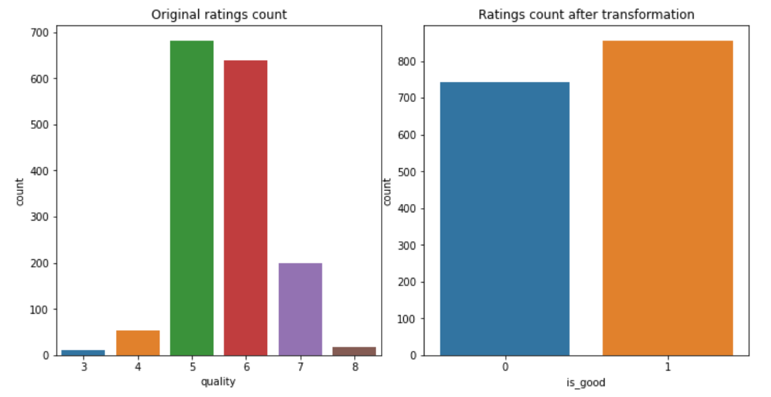
Figure 1.59: Distribution of target before and after transformation
1.4.3.2 Machine learning algorithms used
In order to look at the nature of this data, four well-known algorithms have been trained from data divided into: 1199 observations for the training set and 400 for the test set.
XGBoost (gbm) - powerful modern method based on AdaBoost and gradient boosting, imported from xgboost package, with tuned hyperparameters using the randomized search method from sklearn package, with the best values obtained: min_child_weight - 1, max_depth - 12, learning_rate - 0.05, gamma - 0.2 and colsample_bytree - 0.7
Support Vector Machine (svm) - algorithm, in which we plot each data item as a point in n-dimensional space (where n is number of features) with the value of each feature being the value of a particular coordinate. Then, we perform classification by finding the hyper-plane that differentiates the two classes very well; imported from sklearn package, with tuned hyperparameters using the grid search method from sklearn package, with the best values obteined: C - 10000, gamma - 0.0001 and kernel - rbf
Random Forest (rfm) - method building multiple decision trees and merges them together to get a more accurate and stable prediction; imported from sklearn package, with tuned hyperparameters using the randomized search method from sklearn package4, with the best values obtained: n_estimators - 2000, min_samples_split - 2, min_samples_leaf - 2, max_features - auto, max_depth - 100 and bootstrap - True
Gradient Boosting (xgm) - a type of machine learning boosting. It relies on the intuition that the best possible next model, when combined with previous models, minimizes the overall prediction error; imported from sklearn package, with tuned hyperparameters using the grid search method from sklearn package, with the best values obteined: learning_rate - 0.1, max_depth - 7 and n_estimators - 50
All methods have been implemented in Python with random states set to 42. The choice of these methods was made on the basis of their popularity, diversity and practicality, taking into account the essence of the problem under consideration.
After checking the operation of the models on the test set, the following quality measures were obtained:
| algorithm | accuracy | precision | recall | ROC AUC |
|---|---|---|---|---|
| XGBoost | 0.8050 | 0.806306 | 0.836449 | 0.802633 |
| Support Vector Machine | 0.7475 | 0.798942 | 0.705607 | 0.750653 |
| Random Forest | 0.7850 | 0.801887 | 0.794393 | 0.784293 |
| Gradient Boosting | 0.8075 | 0.818605 | 0.822430 | 0.806376 |
1.4.4 Global explanations
1.4.4.1 Permutation-based variable importance
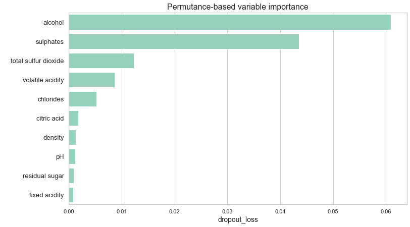
Figure 1.60: Permutation-based variable importance plot for tuned XGBoost model. In this case, size of the bar indicates the positive impact that a feature has on accuracy of the model
Our starting point was rendering a permutation-based variable importance plot from DALEX package using our XGBoost model to examine which variables play the biggest role in model’s decision (Baniecki et al. 2020a). The goal of this method is to inspect which variables have positive impact on the accuracy of the prediction. Surprisingly, all of them seemed to provide information that benefited the accuracy of the model. This, combined with a relatively small size of our dataset, led us to decision not to exclude any variables in further proceedings. However, the importance of the variables varies greatly - alcohol and sulphates together overcome all other factors combined.
1.4.4.2 Mean absolute SHAP value
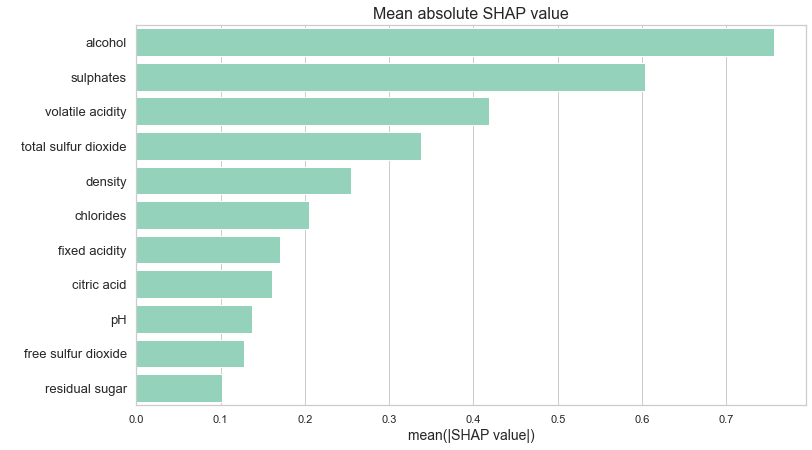
Figure 1.61: Mean absolute SHAP value for tuned XGBoost model. Size of the bar indicates how much a feature influences the prediction on average
In order to gain a different perspective, we examined a plot of mean absolute SHAP values of our model (Scott M. Lundberg and Lee 2017). SHAP method is explained in chapter Break Down and Shapley Additive Explanations (SHAP). Mean absoulte SHAP value can give us insight into which variables influence the predictions the most. Although this method differs significantly from the above-mentioned permutation-based variable importance, it provided us with a similar information on the hierarchy of importance of the variables - once again, alcohol seems to be the biggest factor, followed by sulphates. Analysing those plots encouraged us to take a closer look at the role that alcohol content plays on the prediction.
1.4.4.3 PDP
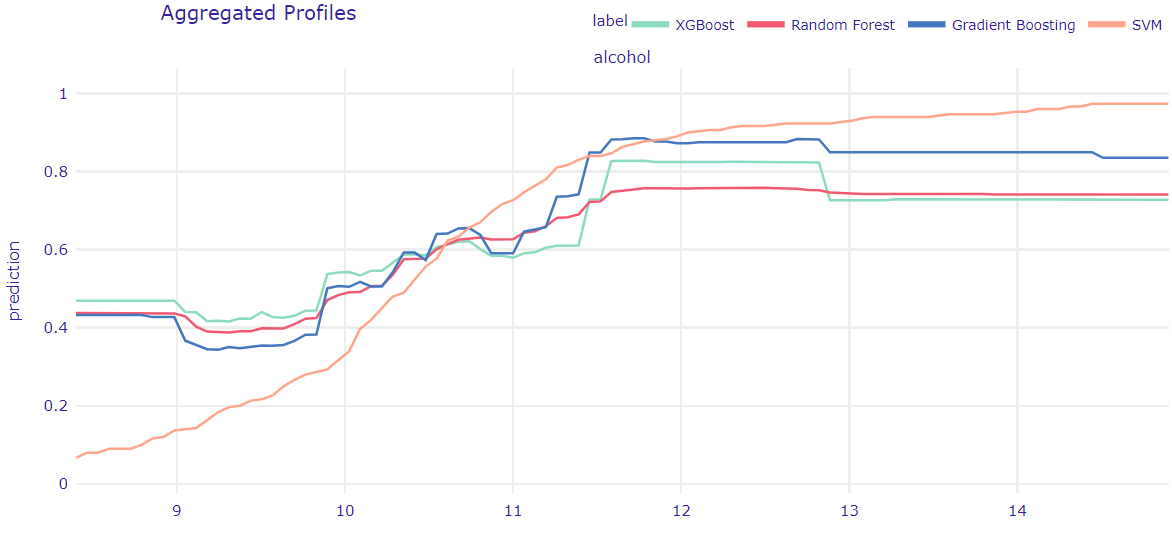
Figure 1.62: Partial Dependence Plot for all models. Lines represent the average prediction by the model if all observations had a fixed value of a feature, in this case - alcohol content
Next, we used Partial Dependence Plot from DALEX package (Baniecki et al. 2020a) to examine an overall effect the alcohol content has on our predictions. PDP tells us what would the average prediction be, if all observations had a fixed value of certain variable. This time, we used all of our models. As expected, tree-based model (XGBoost, GradientBoosting and Random Forest) behave very similarly, while SVM stands out from the rest. However, the main trend is the same - generally, stronger wines are more likely to be good than the weaker ones. Most models reach their lows at just below 10% alcohol content and plateau around 12%.
We have to keep in mind that our data contains only one wine that exceeds 14% alcohol content, which may explain the flat line after that mark for tree-based models. It should be noted that this strongest wine was actually ranked as not good. The fact that the line representing SVM model keeps increasing in value throughout the whole range may indicate that this model is more prone to outliers and doesn’t capture complex interactions as well as other models. It coincides with our prior knowledge of the models and the accuracy scores they achieved.
1.4.4.4 ALE
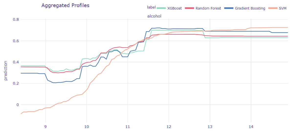
Figure 1.63: Accumulated Local Effects Plot for all models. Lines represent how predictions change in a small range around the value of a feature, in this case - alcohol content.
In order to take into account possible interactions concerning our variable, we generated an ALE plot using all of the models (D. W. Apley and Zhu 2020). This methods shows us how model predictions change in a small “window” of the feature around certain value for data instances in that window. The results turned out to be quite similar to PDP. It makes sense, considering the fact that our dataset doesn’t contain many strongly corelated variables, and the one that is related the most to alcohol, the density, doesn’t have a very significant impact on the predictions made by the models. The most visible difference is probably the way SVM behaves for the biggest alcohol values - it doesn’t seem to differ as much from the other models as in the previous plot.
1.4.5 Local explanations
1.4.5.1 Break Down and Shapley Additive Explanations (SHAP)
The first method that we have used for our local explanations is Shapley Additive Explanations (SHAP). It is based on another explanatory method called Break-Down, which similarly to SHAP is used to compute variables’ attribution to the model’s prediction (Staniak and Biecek 2018a). Break-Down method fixes values of variables in sequence and looks at changes in label value. Moreover, as we can see in figure Figure 1.64 this method is sensitive to the order of variables.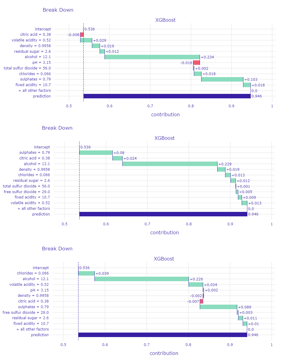
Figure 1.64: BreakDown plots for one observation with different order of fixed variables. Size and color of bars indicates changes in model’s predictions.
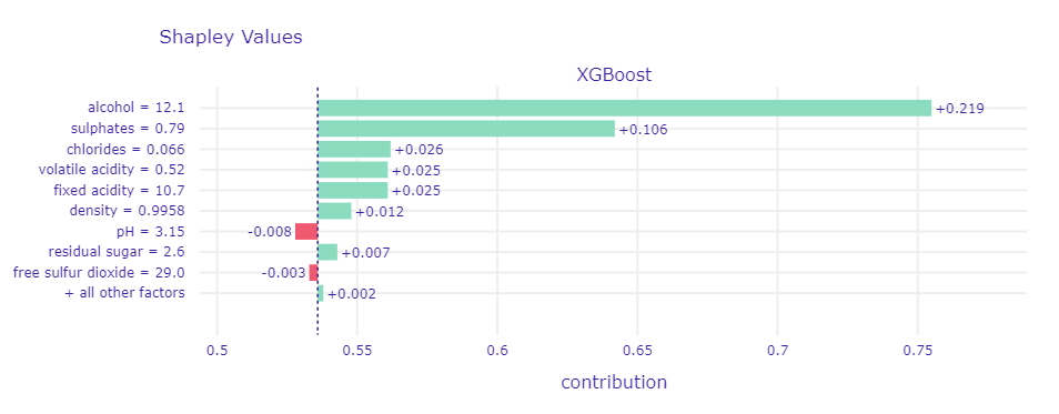
Figure 1.65: Plot of Shapley Values for good wine. Size and color of bars indicates mean change in model’s prediction over different orders of fixed variable.
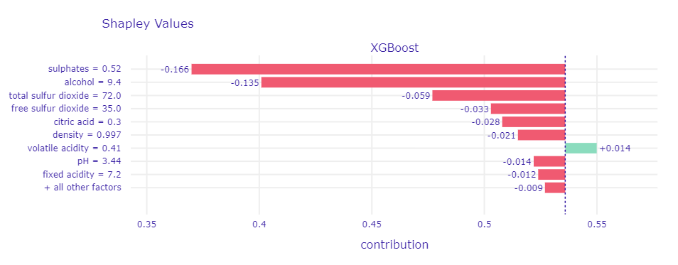
Figure 1.66: Plot of Shapley Values for bad wine.
1.4.5.2 LIME
In order to look at the explainability of individual predictions, the LIME method from DALEX package was used (Baniecki et al. 2020a). When looking at individual visualizations, it is easy to see that extreme alcohol values have the greatest impact on the prediction value. This is clearly visible on the example of incorrectly classified observations - in a significant number of cases it is the non-standard value of alcohol that largely determines the incorrect prediction. The situation is well illustrated by visualizations generated on the basis of two observations which all of our models misclassified.
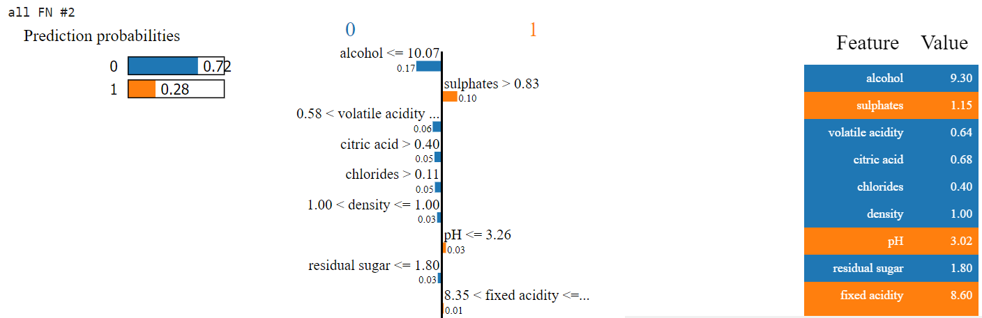
Figure 1.67: Visualization of LIME method for wine incorrectly classified as bad. Left section represents prediction probability. Middle section displays importance of features and right section their exact values. Blue color indicates that variable is supporting class 0 (bad wine) and orange that variable is supporting class 1 (good wine).
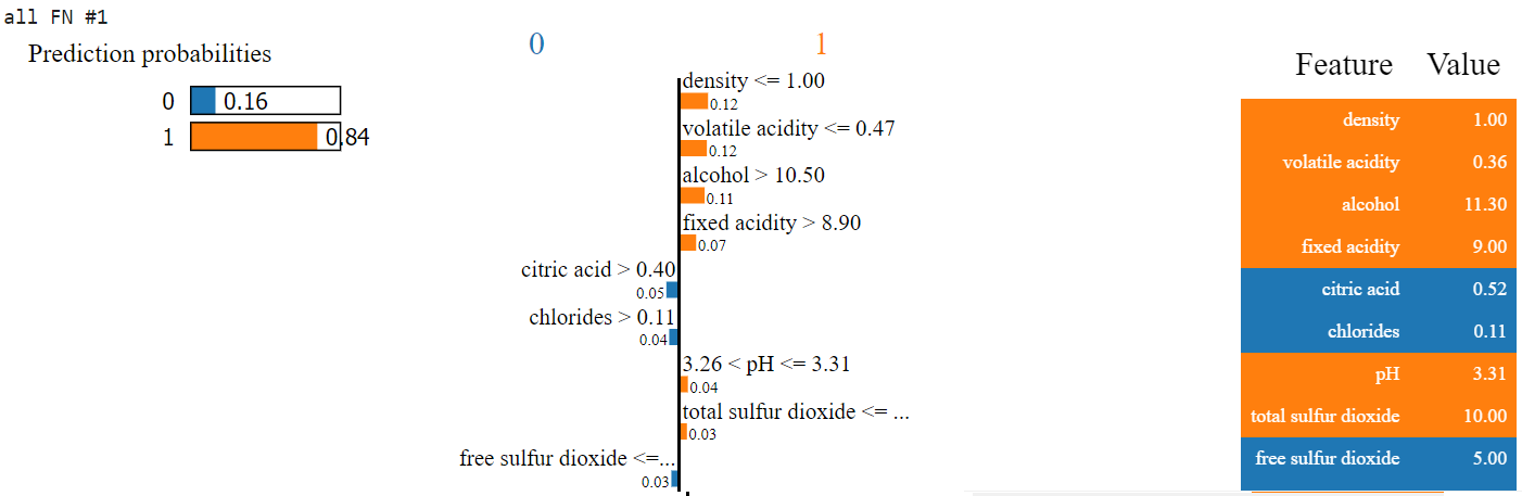
Figure 1.68: Visualization of LIME method for wine incorrectly classified as good.
However, in this case, alcohol does not always dominate, and the prediction result for the XGBoost model is indeed a component of many elements. However, it has to be considered that the LIME method in this case takes into account only certain automatically selected intervals, which, when combined, do not fully represent the essence of the algorithm.
1.4.5.3 Ceteris Paribus
Analyzing results from LIME brought to light yet another issue. Is it possible to change wine’s rating by altering the alcohol content? Answers to this question were provided by a method called Ceteris Paribus. “Ceteris paribus” is a Latin phrase meaning “other things held constant” which accurately describes the main concept of method. Ceteris Paribus illustrates the response of a model to changing a single variable while fixing the values of others. As an example, we will use observation from the previous section which our model incorrectly labeled as the bad one. We quietly assumed that it was due to low alcohol content, but now we can verify our thesis.
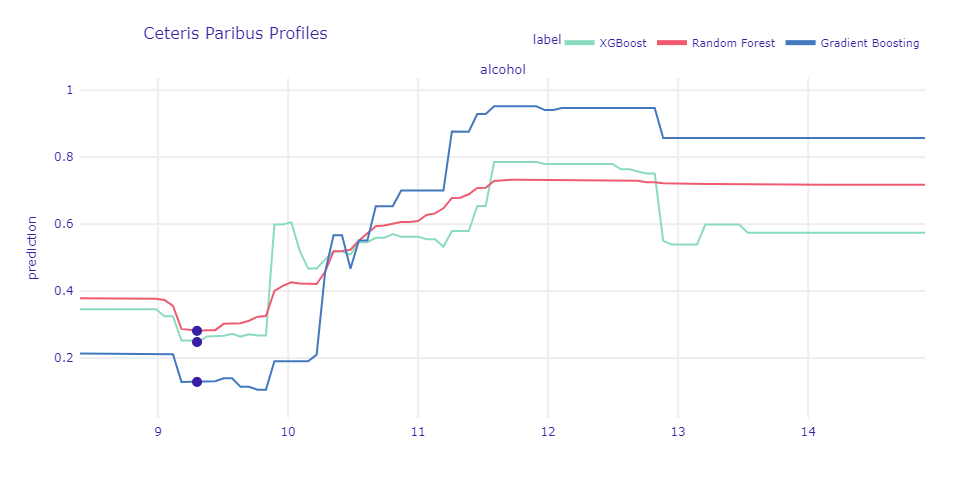
Figure 1.69: Ceteris-paribus profile for all models. Lines represent how the models’ predictions change over different alcohol contents while keeping other variables fixed. Dots represents actual value of alcohol content in examined misclassified wine.
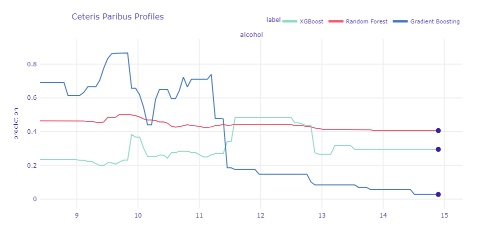
Figure 1.70: Ceteris-paribus profile for alcohol content in a very strong wine.
1.4.6 Confrontation with science
The subject of the quality of wines in relation to their alcohol content has been studied many times before by other scientists and enologists. The topic was covered, among others, on a post on Cult wines blog (England 2019). In 2019, the author pointed that “It is true that alcohol in wine tends to draw out more intense, bold flavours, so the higher the alcohol level, the fuller the body.” Certainly, the phenomenon is also confirmed by the popular fact of preferences of esteemed former wine critic Robert Parker, who was well known for awarding higher scores to higher alcohol wines. On the other hand, lower alcohol wines tend to offer greater balance and pair better with foods. Hence, too much content is also not an advantage in terms of quality.
The phenomenon was also examined by the newspaper the Seattle Times, which published an article in 2003 entitled Does a higher alcohol content mean it’s a better drinking wine? (Gregutt 2003). The expert emphasizes that higher alcohol is an indication of better ripeness at harvest and fermentation to complete or near-complete dryness. With time, the wines are also getting stronger, which is the result of better vineyard practices, letting the grapes get more “hang time” and more efficient yeasts, which definitely has a positive effect on the quality. Here, however, the argument for not too high alcohol content is also emphasized, due to the fact that wines with more than 15 percent are almost never ageworthy. The high alcohol throws the balance off and is often accompanied by too much oak and too much tannin. These wines are also hard to drink, as they do not match well with most foods.
It is also worth comparing an article from the Decanter website (Jefford 2010) with the results of our study. As a person well acquainted with the subject, the expert considers the alcohol threshold of a good wine, coming to a conclusion consistent with the results of our calculations.
Professional research was conducted in 2015. A group of Portugese experts conducted a thorough research, the result of which was the article From Sugar of Grape to Alcohol of Wine: Sensorial Impact of Alcohol in Wine (Jordão et al. 2015). They indicated in it that the quality of grapes, as well as wine quality, flavor, stability, and sensorial characteristics depends on the content and composition of several different groups of compounds from grapes. One of these groups of compounds are sugars and consequently the alcohol content quantified in wines after alcoholic fermentation. During grape berry ripening, sucrose transported from the leaves is accumulated in the berry vacuoles as glucose and fructose resulting in a fuller taste of a final wine.
The idea of a threshold of an alcohol content, beyond which wines lose their quality, is a common theme in literature dedicated to the topic. There is evidence suggesting that wines that have more than 14.5% of alcohol start to come off as herbaceous instead of fruity (GOLDNER et al. 2009). The research states that the sensory perception of the aroma changed dramatically with the level of ethanol content in the wine, but the change isn’t consistent among all chemical compounds.
Another very interesting topic is the idea of reducing the alcohol content in wine after initial production process (Jordão et al. 2015). Motivation behind such actions is to try to keep all the good aromas and qualities associated with stronger wines, while simultaneously lowering excessive alcohol which causes bitter or sour tastes. Such attempts ended in mixed results, but evidence suggests that it may be possible to lower alcohol content by one percentage point without losing many aromas.
1.4.7 Summary
The analysis of the results of modern methods of explainable artificial intelligence showed a relatively unambiguous conclusion - taking into account the proven data set of popular wines assessed by experts, the alcohol content definitely has a large impact on the average rating of wines. Despite taking into account many different chemical factors, as well as the variety of black box models and the differences between individual observations, alcohol is a factor that stands out from other predictors. This result is evidenced not only by the high correlation and simple conclusions from the visualizations, but also by the results of the algorithms explaining the results of the models used. However, the methodology has produced less obvious conclusions - although higher alcohol content is associated with higher alcohol quality (at least in a pseudo-objective sense), there is a threshold at which this property reverses. These considerations are the result of measuring not only one or two approaches, but a total of research based on as many as seven methods. It is a good argument to appreciate both them and modern solutions of explainable artificial intelligence. Indeed, the results of information and mathematical analysis are also consistent with what we can observe in nature - the effects of the calculations made are consistent with previous research related to the topic, and not necessarily based on methods related to the field of data science.
1.4.8 Conclusions
The experiment is undoubtedly successful and with a high degree of certainty confirms two facts: firstly, the quality of the wines is dependent on their higher alcohol content, but up to a certain threshold and secondly, modern methods of explainable artificial intelligence provides us valuable results that bring new valuable information about the black box models, which at the same time are consistent with the nature of the data sets on which they were made. Different approaches provide us with various useful information and it is difficult to indicate better or worse solutions - the seven methods mentioned complement each other in their own way, but each allows us to look at the problem of analysis from a different perspective.
Leaving aside our succesful implementation of XAI solutions, one must bear in mind, that the results of the experiment need to be put in a certain perspective. It must be remembered that the world of wines is a very diverse one. For example, artificially fortified wines like port wine or sherry should be considered separately. The discussed data set concerns only a certain group of wines and we don’t know enoguh about the experts or conditions of the tastings to call the data entirely representative. Therefore, we should remain cautious when drawing any far-reaching conclusions. Nevertheless, the conducted research approximates the idea of the overall effect of alcohol on the quality of wine and confirms previous research by experts from a biochemical point of view.