3.7 Which Neighbours Affected House Prices in the ’90s?

Authors: Hubert Baniecki, Mateusz Polakowski (Warsaw University of Technology)

3.7.1 Abstract

The house price estimation task has a long-lasting history in economics and statistics. Nowadays, both worlds unite to exploit the machine learning approach; thus, achieve the best predictive results. In the literature, there are myriad of works discussing the performance-interpretability tradeoff apparent in the modelling of real estate values. In this paper, we propose a solution to this problem, which is a highly interpretable stacked model that outperforms the black-box models. We use it to examine neighbourhood parameters affecting the median house price in the United States regions in 1990.

3.7.2 Introduction

Real estate value varies over numerous factors. These may be obvious like location or interior design, but also less apparent like the ethnicity and age of neighbours. Therefore, property price estimation is a demanding job that often requires a lot of experience and market knowledge. Is or was, because nowadays, Artificial Intelligence (AI) surpasses humans in this task (Conway 2018). Interested parties more often use tools like supervised Machine Learning (ML) models to precisely evaluate the property value and gain a competitive advantage (Park and Bae 2015; Rafiei and Adeli 2015; Liu and Liu 2019).

The dilemma is in blindly trusting the prediction given by so-called black-box models. These are ML algorithms that take loads of various real estate data as input and return a house price estimation without giving their reasoning. Black-box complex nature is its biggest strength and weakness at the same time. This trait regularly entails high effectiveness but does not allow for interpretation of model outputs (Baldominos et al. 2018). Because of that, specialists interested in supporting their work with automated ML decision-making are more eager to use white-box models like linear regression or decision trees (Selim 2009). These do not achieve state-of-the-art performance efficiently, but instead, provide valuable information about the relationships present in data through model interpretation.

For many years houses have been popular properties; thus, they are of particular interest for ordinary people. What exact influence had the demographic characteristics of the house neighbourhood on its price in the ’90s? Although in the absence of current technology, it has been hard to answer such question years ago (Din, Hoesli, and Bender 2001), now we can.

In this paper, we perform a case study on the actual United States Census data from 1990 (“Census dataset” 1996) and deliver an interpretable white-box model that estimates the median house price by the region. We present multiple approaches to this problem and choose the best model, which achieves similar performance to complex black-boxes. Finally, using its interpretable nature, we answer various questions that give a new life to this historical data.

3.7.3 Related Work

The use of ML in the real estate domain is a well-documented ground (Conway 2018) and not precisely a topic of this contribution. We relate to the works that aim to use Interpretable ML techniques (Molnar 2019b) to interpret models predictions in the house price estimation problem.

The state-of-the-art approach to house price estimation is to combine linear and semi-log regression models with the Hedonic Pricing Method (Garrod and Willis 1992; Randeniya, Ranasinghe, and Amarawickrama 2017), which aims to determine the extent that environmental or ecosystem factors affect the price of a good. (Özalp and Akinci 2017) deliberately seeks to interpret the outcome and provide information about the parameters that affect property value. There are also comparisons between the linear white-box and black-box models (Selim 2009; Baldominos et al. 2018) which showcase the performance-interpretability tradeoff (Gosiewska and Biecek 2020).

Nature of the topic might entail that data is place-specific; therefore, part of the studies focus on a single location with the use of geospatial data. The case study on London (Law 2017) links the street network community structure with house price, which takes into consideration the topology of the city. In contradiction, (Heyman and Sommervoll 2019) uses the Oslo city data to explore the differences between the relative and absolute location attributes. Applying data like the distance to the nearest shop and transportation is place-agnostic.

One of the new ideas is to utilize location data from multiple sources in a Multi-Task Learning approach (Gao et al. 2019). It also studies the relationships between the tasks, which gives an extensive insight on prediction attributions.

In this paper, we partially aim to enhance the use of regression decision tree models, which had been utilized to estimate the house prices based on their essential characteristics in (Fan, Ong, and Koh 2006).

3.7.4 Data

For this case study we use the house_8L dataset crafted from the data collected in 1990 by the United States Census Bureau. Each record stands for a distinct United States state while the target value is a median house price in a given region. The variables are presented in Table 3.1.

TABLE 3.1: Description of variables present in the house_8L dataset.

Original.name	New.name	Description	Median
price	price	median price of the house in the region	33100
P3	house_n	total number of households	505
H15.1	avg_room_n	average number of rooms in an owner-occupied Housing Units	5.957
H5.2	forsale_h_pct	percentage of vacant Housing Units which are for sale only	0.148
H40.4	forsale_6mplus_h_pct	percentage of vacant-for-sale Housing Units vacant more then 6 months	0.500
P11.3	age_25_64_pct	percentage of people between 25-64 years of age	0.483
P16.2	family_2plus_h_pct	percentage of households with 2 or more persons which are family households	0.714
P19.2	black_h_pct	percentage of households with black Householder	0.003
P6.4	asian_p_pct	percentage of people which are of Asian or Pacific Islander race	0.002

Furthermore, we will apply our Metodology (Section 3.7.5) on a corresponding house_16H dataset, which has the same target but a different set of variables. More correlated variables of a higher variance make it significantly harder to estimate the median house price in a given region. Such validation will allow us to evaluate our model on a more demanding task. The comprehensive description of used data can be found in (“Census dataset” 1996).

3.7.5 Methodology

In this section, we are going to focus on developing the best white-box model, which provides interpretability of features. Throughout this case study, we use the Mean Absolute Error (MAE) measure to evaluate the model performance, because we focus on the residuals while the mean of absolute values of residuals is the easiest to interpret.

3.7.5.1 Exploratory Data Analysis

Performing the Exploratory Data Analysis highlighted multiple vital issues with the data. Firstly, Figure 3.7 presents the immerse skewness of the target, which usually leads to harder modelling. However, we decided not to transform the price variable because this might provide less interpretability in the end. Secondly, there are 46 data points with unnaturally looking target value. We suspect that the target value of 500001 is artificially made, so we removed these outliers. Finally, there are six percentage and two count variables, which indicates that there are not many possibilities for feature engineering.

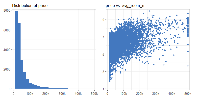
FIGURE 3.7: (L) Histogram of the target values shows that the distribution is very skewed. (R) Exemplary variable correlation with the target shows that there are few data points with the same, unnaturally high target value.

It is also worth noting that there are no missing values and the dataset has over 22k data points which allow us to reliably split the data into train and test subsets using the 2:1 ratio. Throughout this case study, we use the Mean Absolute Error (MAE) measure to evaluate the model performance, because we later focus on the residuals while the mean of absolute values of residuals is the easiest to interpret.

3.7.5.2 SAFE

The first approach was using the SAFE (Gosiewska et al. 2019) technique to engineer new features and produce a linear regression model. We trained a well-performing black-box ranger (Wright and Ziegler 2017) model and extracted new interpretable features using its Partial Dependence Profiles (Friedman 2000). Then we used these features to craft a new linear model which indeed was better than the baseline linear model by about 10%. It is worth noting that both of these linear models had a hard time succeeding because of the target skewness.

3.7.5.3 Divide-and-conquer

In this section, we present the main contribution of this paper. The divide-and-conquer idea has many computer science applications, e.g. in sorting algorithms, natural language processing, or parallel computing. We decided to make use of its core principles in constructing the method for fitting the enhanced white-box model. The final result is multiple tree models combined which decisions are easily interpretable.

The proposed algorithm presented in Figure 3.8 is:

1. Divide the target variable with k middle points into k+1 groups.
2. Fit a black-box classifier on train data which predicts the belonging to the i-th group.
3. Use this classifier to divide the train and test data into k+1 train and test subsets.
4. For every i-th subset fit a white-box estimator of target variable on the i-th train data.
5. Use the i-th estimator to predict the outcome of the i-th test data.

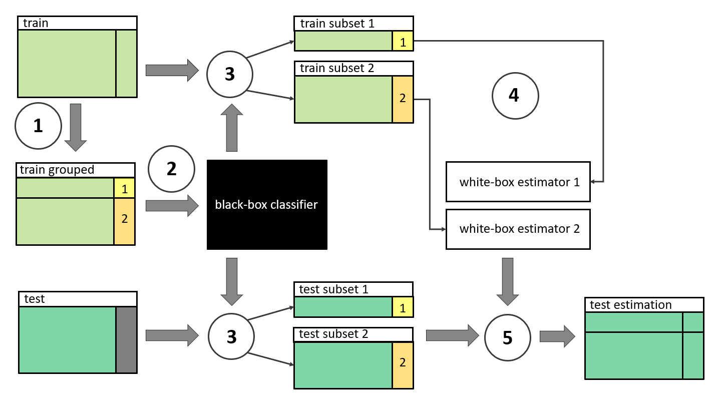
FIGURE 3.8: Following the steps 1-5 presented in the diagram, the divide-and-conquer algorithm is used to construct an enhanced white-box model. Such a stacked model consists of the black-box classifier and white-box estimators.

The final product is a stacked model with one classifier and k+1 estimators. The exact models are for engineers to choose. It is worth noting that the unsupervised clustering method might be used instead of the classification model.

3.7.6 Results

3.7.6.1 The stacked model

For the house price task, we chose k = 1, and the middle point was arbitrary chosen as 100k, which divides the data into two groups in about a 10:1 ratio. We used the ranger random forest model as a black-box classifier and the rpart (Therneau and Atkinson 2019b) decision tree model as a white-box estimator.

The ranger model had default parameters with mtry = 3. The parameters of rpart models were:

• maxdepth = 4 - low depth reassures the interpretability of the model
• cp = 0.001 - lower complexity helps with the skewed target
• minbucket = 1% of the training data - more filled tree leaves adds up to higher interpretability

Figure 3.9 depicts the tree that estimates cheaper houses, while Figure 3.10 presents the tree that estimates more expensive houses.

FIGURE 3.9: The tree that estimates cheaper houses. Part of the stacked model.

FIGURE 3.10: The tree that estimates more expensive houses. Part of the stacked model.

Interpreting the stacked model presented in Figures 3.9 & 3.10 leads to multiple conclusions. Firstly, we can observe the noticeable impact of features like the total number of households or the average number of rooms on the median price of the house in the region, which is compliant with basic intuitions. It is also evident that the bigger percentage of people between 25-64 years of age the higher the prices.

Finally, we can observe the impact of critical features. The percentage of people which are of Asian or Pacific Islander race divides the prices in an opposing direction to the percentage of households with black Householder. The corresponding tree splits showcase which neighbours, and in what manner, affected house prices in the ’90s. Whether it is a correlation or causality is a valid debate that could be further investigated.

3.7.6.2 Comparison of the residuals

In this section, we compare our stacked model with baseline ranger and rpart models, respectively referred to as black-box and white-box. Our solution achieves competitive performance with interpretable features.

The main idea behind the divide-and-conquer technique was to minimize the maximum value of the absolute residuals, which reassures that no significant errors will happen. Such an approach may inevitably lead to minimizing the sum of the absolute residual values (MAE). In Figure 3.11, we can see that the targets mentioned above were indeed met. The stacked model not only has the lowest maximum error value but also has the best performance on average, as the red dot highlights the MAE score.

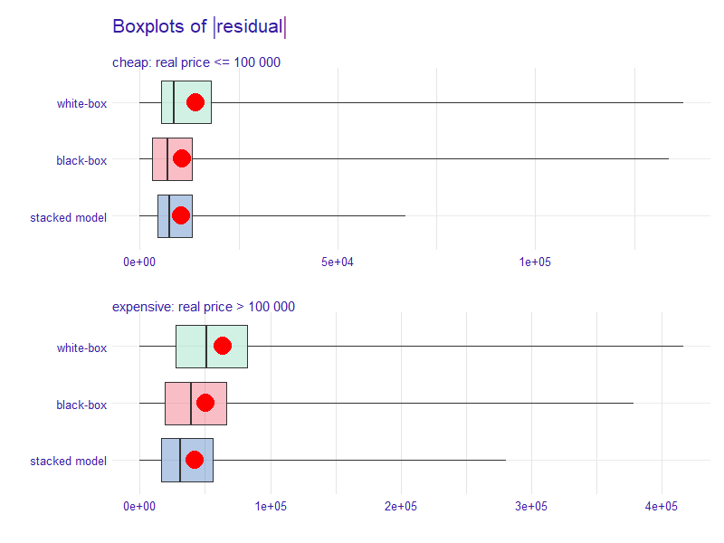
FIGURE 3.11: Boxplots of residuals for the stacked model compared to black-box and white-box models. The plot is divided for cheaper and more expensive houses. The red dot highlights the MAE score.

Figure 3.12 presents a more in-depth analysis of model residuals. In the top, we can observe that the black-box model has the lowest absolute residual mode (tip of the distribution), but the stacked model lays more in the centre (base of the distribution), which leads to more even spread of residuals. In the bottom, we can observe that the black-box model tends to undervalue house prices, while our model overestimates them. Looking at the height of the tip of the distribution and its shape, we can conclude that the stacked model provides more reliable estimations.

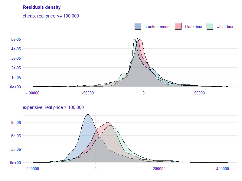
FIGURE 3.12: Density of residuals for the stacked model compared to black-box and white-box models. The plot is divided for cheaper and more expensive houses.

3.7.6.3 Comparison of the scores

Finally, we present the comparison of MAE scores for all of the used models in this case study in Table 3.2. There are two tasks with different variables, complexity and correlations. We calculate the scores on the test subsets.

We can see that the linear models performed the worse, although the SAFE approach noticeably lowered the MAE. Then there is a decision tree which performed better but not so on the more laborious task. Both of the black-box models did a far better job at house price estimation than interpretable models. Finally, our stacked model is a champion with the best performance on both of the tasks.

TABLE 3.2: Comparison of the MAE score for all of the used models on test datasets. Light colour highlights white-box models, while the dark colour is for black-box models.

	Dataset (test)
Model	house_8L	house_16H
linear model	23.1k	24.1k
SAFE on ranger	21.4k	22.6k
rpart	19.2k	22.1k
xgboost	16k	16.5k
ranger	14.8k	15.6k
stacked model	14.6k	15.3k

3.7.7 Conclusions

This case study aimed to provide an interpretable machine learning model that achieves state-of-the-art performance on the datasets crafted from the data collected in 1990 by the United States Census Bureau. We not only provided such a model but also examined its decision-making process to determine how it estimates the median house price in the United States regions. The stacked model had prominently shown the impact of neighbours’ age and race in predicting the outcome.

We believe that the principles of the divide-and-conquer algorithm can be successfully applied in other domains to neglect the performance-interpretability tradeoff apparent while using machine learning models. In further research, we would like to generalize this approach into a well-defined framework and apply it to several different problems.

References

Baldominos, Alejandro, Iván Blanco, Antonio Moreno, Rubén Iturrarte, Óscar Bernárdez, and Carlos Afonso. 2018. “Identifying Real Estate Opportunities Using Machine Learning.” Applied Sciences 8 (November): 2321. https://doi.org/10.3390/app8112321.

“Census dataset.” 1996. http://www.cs.toronto.edu/~delve/data/census-house/censusDetail.html.

Conway, Jennifer. 2018. “Artificial Intelligence and Machine Learning : Current Applications in Real Estate.” PhD thesis. https://dspace.mit.edu/bitstream/handle/1721.1/120609/1088413444-MIT.pdf.

Din, Allan, Martin Hoesli, and André Bender. 2001. “Environmental Variables and Real Estate Prices.” Urban Studies 38 (February). https://doi.org/10.1080/00420980120080899.

Fan, Gang-Zhi, Seow Eng Ong, and Hian Koh. 2006. “Determinants of House Price: A Decision Tree Approach.” Urban Studies 43 (November): 2301–16. https://doi.org/10.1080/00420980600990928.

Friedman, Jerome. 2000. “Greedy Function Approximation: A Gradient Boosting Machine.” The Annals of Statistics 29 (November). https://doi.org/10.1214/aos/1013203451.

Gao, Guangliang, Zhifeng Bao, Jie Cao, A. Qin, Timos Sellis, Fellow, IEEE, and Zhiang Wu. 2019. “Location-Centered House Price Prediction: A Multi-Task Learning Approach,” January. https://arxiv.org/abs/1901.01774.

Garrod, Guy D, and Kenneth G Willis. 1992. “Valuing Goods’ Characteristics: An Application of the Hedonic Price Method to Environmental Attributes.” Journal of Environmental Management 34 (1): 59–76. https://doi.org/10.1016/S0301-4797(05)80110-0.

Gosiewska, Alicja, and Przemyslaw Biecek. 2020. “Lifting Interpretability-Performance Trade-off via Automated Feature Engineering.” https://arxiv.org/abs/2002.04267.

Gosiewska, Alicja, Aleksandra Gacek, Piotr Lubon, and Przemyslaw Biecek. 2019. “SAFE Ml: Surrogate Assisted Feature Extraction for Model Learning.” http://arxiv.org/abs/1902.11035.

Heyman, Axel, and Dag Sommervoll. 2019. “House Prices and Relative Location.” Cities 95 (September): 102373. https://doi.org/10.1016/j.cities.2019.06.004.

Law, Stephen. 2017. “Defining Street-Based Local Area and Measuring Its Effect on House Price Using a Hedonic Price Approach: The Case Study of Metropolitan London.” Cities 60 (February): 166–79. https://doi.org/10.1016/j.cities.2016.08.008.

Liu, Rui, and Lu Liu. 2019. “Predicting housing price in China based on long short-term memory incorporating modified genetic algorithm.” Soft Computing, 1–10. https://doi.org/10.1007/s00500-018-03739-w.

Molnar, Christoph. 2019b. Interpretable Machine Learning: A Guide for Making Black Box Models Explainable. https://christophm.github.io/interpretable-ml-book/simple.html.

Özalp, Ayşe, and Halil Akinci. 2017. “The Use of Hedonic Pricing Method to Determine the Parameters Affecting Residential Real Estate Prices.” Arabian Journal of Geosciences 10 (December). https://doi.org/10.1007/s12517-017-3331-3.

Park, Byeonghwa, and Jae Bae. 2015. “Using machine learning algorithms for housing price prediction: The case of Fairfax County, Virginia housing data.” Expert Systems with Applications 42 (April). https://doi.org/10.1016/j.eswa.2014.11.040.

Rafiei, Mohammad H., and Hojjat Adeli. 2015. “A Novel Machine Learning Model for Estimation of Sale Prices of Real Estate Units.” Journal of Construction Engineering and Management 142 (August). https://doi.org/10.1061/(ASCE)CO.1943-7862.0001047.

Randeniya, TD, Gayani Ranasinghe, and Susantha Amarawickrama. 2017. “A model to Estimate the Implicit Values of Housing Attributes by Applying the Hedonic Pricing Method.” International Journal of Built Environment and Sustainability 4 (May). https://doi.org/10.11113/ijbes.v4.n2.182.

Selim, Hasan. 2009. “Determinants of House Prices in Turkey: Hedonic Regression Versus Artificial Neural Network.” Expert Syst. Appl. 36 (March): 2843–52. https://doi.org/10.1016/j.eswa.2008.01.044.

Therneau, Terry, and Beth Atkinson. 2019b. Rpart: Recursive Partitioning and Regression Trees. https://CRAN.R-project.org/package=rpart.

Wright, Marvin N., and Andreas Ziegler. 2017. “ranger: A Fast Implementation of Random Forests for High Dimensional Data in C++ and R.” Journal of Statistical Software 77 (1): 1–17. https://doi.org/10.18637/jss.v077.i01.