A word about black boxes

Nowadays a fierce competition can be observed – scientists are surpassing each other in creating better regression models. As those models are getting more complex, it is becoming almost impossible to illustrate results relation with data, in a way humans understand. They are commonly called ‘black boxes’. ‘Machine learning is frequently referred to as a black box—data goes in, decisions come out, but the processes between input and output are opaque’ ~ The Lancet. Despite their excellent performance, sometimes models with easily interpretable output can be more desired, e.g. in banking.

What can be done?

Results ready for further human analysis can be achieved with explainable models (linear models, decision trees, etc.) and adequate data preparation. This subject was taken up by the Warsaw University of Technology students in their brilliant article. Their experiments were conducted using ‘eucalyptus’ OpenML dataset. The target variable is a utility with values: ‘low’, ‘average’, ‘good’, and ‘best’. To compare models authors used AUC measure, which can is represented as an area under the ROC curve.

Black box vs white box

As a representative model of black boxes, the extreme gradient boosting algorithm was chosen. The authors compared it with the tree model. To improve white box performance, the following actions were taken:

• splitting a 4-class classification problem into 3 binary classification problems
• transforming the target variable into numeric values
• imputing missing data in the training set
• selecting variables
• transforming variable

Results

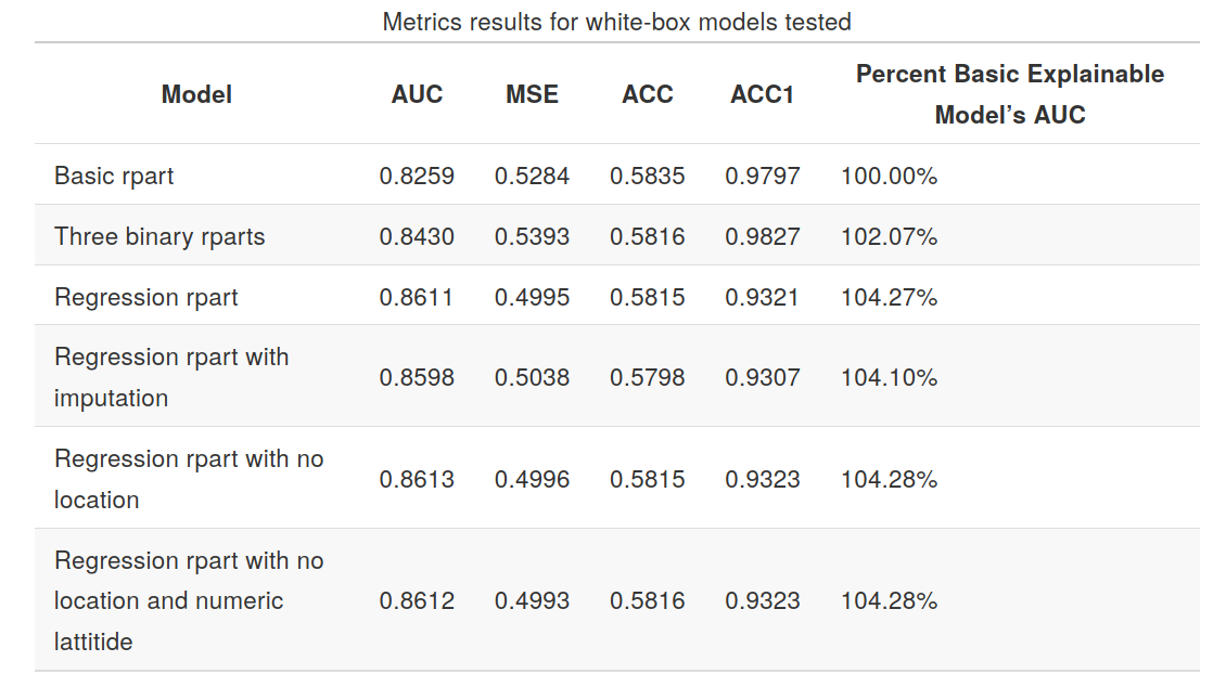
The results are shown in the tables below.

Explainable models:

Black box models:

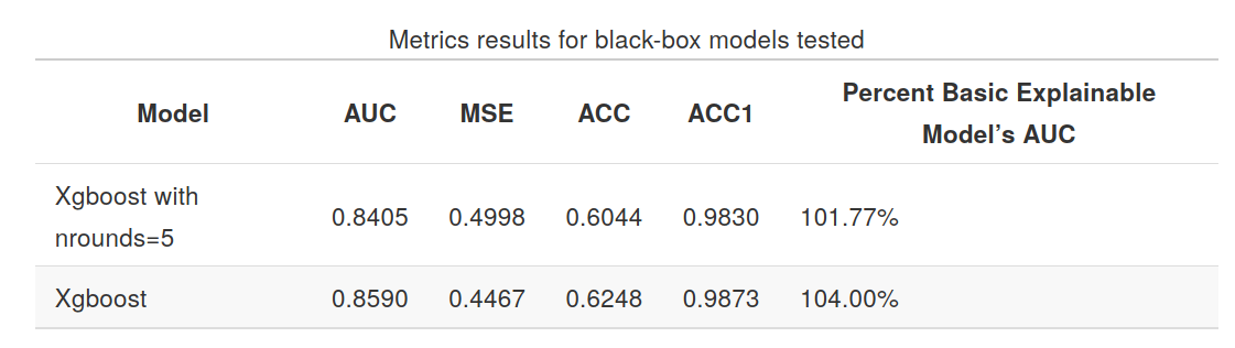
As presented on charts, the best result was obtained by explainable model - decision tree with selected variables.

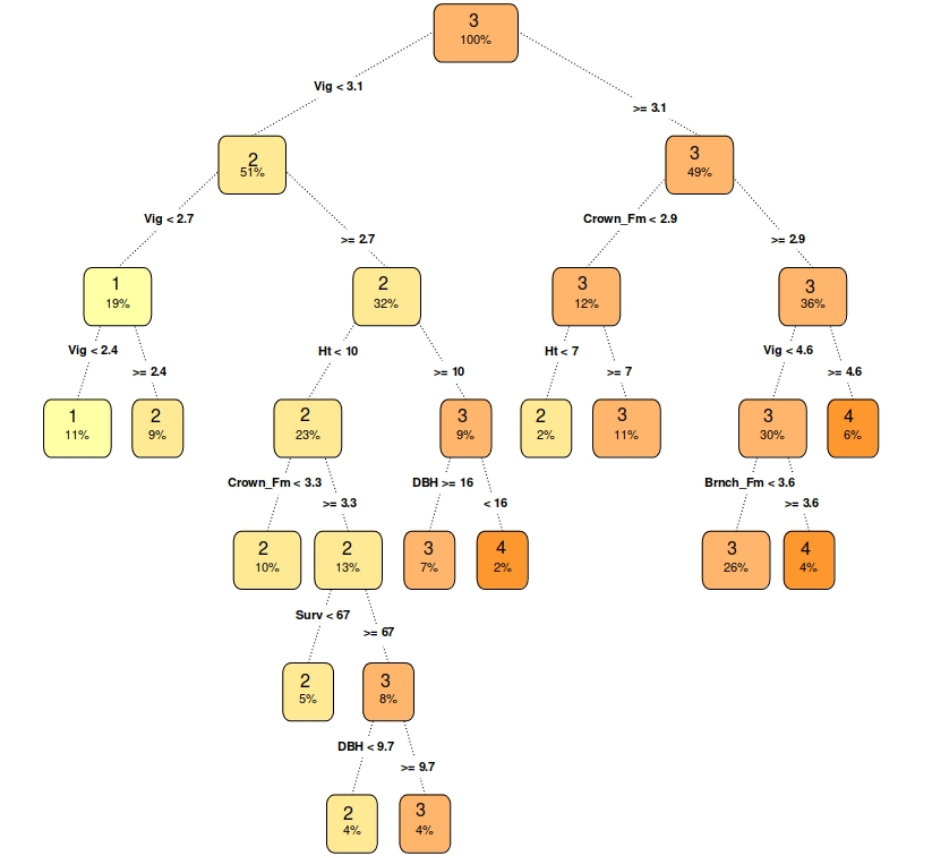
So, how can we explain the final model?

As previously stated, the model that outperformed the competition is a simple decision tree regression, which can be quite easily shown on a tree plot. The plot is interpreted, by starting in the root node and going to the next nodes via edge which suits our observation. At the end of this path can be found a leaf with the predicted value.

Conclusion

Authors’ research proved that black boxes are not always the best performing models and with some effort, the easily explainable output can be achieved. Surely, the discussed dataset was not a complicated machine learning problem, but the described article is very informative and the results are thought-provoking.