Prepare to fight
The interpretability of machine learning models is gaining more and more interest in the scientific world. It’s because artificial intelligence is used in a lot of business solutions that impact our everyday life. Knowledge how the model works can, among others, assure us about the safety of the implemented solution. We came across the article of students of the Warsaw University of Technology Wojciech Bogucki, Tomasz Makowski, Dominik Rafacz titled “Predicting code defects using interpretable static measures.” touching this topic.

Black box vs white box
Using interpretable models, such as linear regression, decision trees and k-nearest neighbors is one way to have your solution explainable. Authors of the discussed article checked if applying different transformations to the dataset can help white-box models outperform black-box models. They were trying to predict code defects of C and C++ functions basing on the dataset describing the functions in terms of simple measures, like for example length of the code and number of operands. The Black-box model they were trying to beat was random forest with default hyperparameters.
Exchange of blows
They were trying to improve their white-box models of choice in consecutive stages. In every stage, they compared results of applying several upgrades of similar character to their solutions and then decided whether to keep any of them. Every step of this work is presented in the table below:
| Order | Applied operation | logreg | kknn | rpart | Kept? |
|---|---|---|---|---|---|
| - | Base | $0.735$ | $0.728$ | $0.500$ | - |
| 0 | rpart tuning |
$0.735$ | $0.728$ | $0.737$ | yes |
| 1a | Normalization | $0.735$ | $0.727$ | $0.737$ | no |
| 1b | Outlier reduction | $0.743$ | $0.732$ | $0.739$ | no |
| 1c | Logarithm | $0.744$ | $0.718$ | $0.725$ | no |
| 2a | Outlier reduction and normalization | $0.743$ | $0.732$ | $0.739$ | yes |
| 2b | Logarithm and outlier reduction | $0.744$ | $0.717$ | $0.725$ | no |
| 3a | Gain-ratio discretization | $0.743$ | $0.732$ | $0.739$ | no |
| 3b | rSAFE |
$0.744$ | $0.718$ | $0.734$ | no |
| 4a | New features selected by ranger |
$0.747$ | $0.729$ | $0.733$ | no |
| 4b | New features selected by rpart |
$0.745$ | $0.731$ | $0.739$ | no |
| 4c | Halstead’s measures | $0.745$ | $0.731$ | $0.738$ | no |
| 5a | SMOTE with new features by ranger |
$0.749$ | $0.737$ | $0.800$ | no |
| 5b | SMOTE with new features by rpart |
$0.747$ | $0.736$ | $0.793$ | no |
| 5c | SMOTE without new features |
$0.745$ | $0.736$ | $0.804$ | yes |
They decided to use AUC to assess the quality of models (values in columns logreg, kknn, rpart). The dataset was imbalanced (only 20% observations were code with defects) and AUC is not the most suitable for imbalanced data but according to authors 20%/80% still is not a tragedy. We wonder what would be if they used different measures, such as the Matthews correlation coefficient.
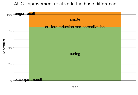
The first step they made was hyperparameter tuning of the decision tree. It produced the most drastic gain of all the steps. Before it, the decision tree was only as good as random assignment, and just after tuning it slightly overtaken other white-boxes. Maybe in the case of black-box random forest, tuning would have also brought a big improvement. Such a pity, the authors didn’t discuss it. Hyperparameter tuning does not need a lot of effort and is almost always done also with the random forest.
The authors also considered the discretization of columns as a way to improve results. Unfortunately, the techniques they used didn’t bring any improvement. Looking at the partial dependence plot produced with the DALEX package they concluded that there is no variable to be discretized, probably because of no linear dependency of variables.
An important part of their aim was to check whether Halstead’s and McCabe’s measures were reliable. Adding Halstead’s measures did not bring any significant improvement and so the authors concluded his hypothesis was wrong. They were not able to remove McCabe’s measures from the set and so were not able to test their validity. Maybe checking the importance of McCabe’s measures would be a good idea to check how they contribute to the result - how important they are compared to basic features and do they contribute in the same direction as their author intended to.
Fair victory?
Finally, the authors managed to upgrade the decision tree so it has beaten random forest. Although, the main thing contributing to this was hyperparameter tuning. The authors were rather not satisfied with this result.

To sum up, in our opinion, it’s a crucial topic and good that somebody is creating such things. It’s a pity that authors were not able to get more out of the dataset transformations, especially Halstead’s and McCabe’s measures. Questions, which are intriguing for us, are if they were able to beat random forest with tuned hyperparameters or other black-box models, such as XGBoost or LightGBM.